“不积跬步无以至千里。”
前言
快速排序 worst-case 的时间复杂度是 \(Θ(n^2)\)。
由于其平均性能很好,期望时间复杂度是 \(Θ(n lgn )\)。
所以是实际排序应用中最好的选择。
快速排序采用了一种分治的策略,通常称其为分治法( Divide-and-Conquer Method )。
描述
分治法的基本思想是:
将原问题分解为若干个规模更小但结构与原问题相似的子问题。
递归地解这些子问题,然后将这些子问题的解组合为原问题的解。
主要分三步:
-
分( divide )
选定主元( pivot ) A[q]。
将数组 A[p…r] 划分成两个子数组 A[p…q−1] 和 A[q+1…r]。
使得 A[p…q−1] 的元素均小于A[q],而 A[q+1…r] 的元素不小于 A[q]。 -
治( conquer )
递归地排序两个子数组。 -
combine
实际上,子数组是原址排序的,不需要合并操作。
分区( partition )解析
快速排序的关键是分区,下面说一下分区步骤:
1> 在数据集之中,选择一个元素作为「基准」(pivot)。
2> 所有小于「基准」的元素,都移到「基准」的左边;
所有大于「基准」的元素,都移到「基准」的右边。
这个操作称为分区 ( partition ) 操作,分区操作结束后,
基准元素所处的位置就是最终排序后它的位置。
3> 对”基准”左边和右边的两个子集,不断重复第一步和第二步,直到所有子集只剩下一个元素为止。
伪代码如下:
function partition(a, left, right, pivotIndex)
     pivotValue := a[pivotIndex]
     swap(a[pivotIndex], a[right]) // 把 pivot 移到末尾
     storeIndex := left
     for i from left to right-1
         if a[i] < pivotValue
             swap(a[storeIndex], a[i])
             storeIndex := storeIndex + 1
     swap(a[right], a[storeIndex]) // 移动 pivot 到最终的位置
     return storeIndex // 返回 pivot 的最终位置
首先,把基准元素移到末尾(如果直接选择最后一个元素为基准元素,那就不用移动)。
然后从左到右(除了最后的基准元素),循环移动小于等于 pivot 的元素到数组的开头,
每次移动, storeIndex 自增 1,表示下一个小于 pivot 的元素将要移动到的位置。
循环结束后 storeIndex 所代表的的位置就是 pivot 最终的位置。
所以最后将 pivot 所在位置(此时是右侧)与 storeIndex 所代表的的位置的元素交换位置。
要注意的是,一个元素在到达它的最后位置前,可能会被交换很多次。
实例分析
现有数组 arr = [6, 10, 13, 5, 8, 3, 5, 2, 11]
1> 首先选定 pivot element,比如选择 5
                      pivot
                        ↓
6   10  13  5   8   3   5   2   11
2> 交换 pivot 与最后一个元素的位置(若选择最后一个为基准元素,则此步省略)。
                               pivot
                                 ↓
6   10  13  5   8   3   11   2   5
3> 循环从左至右(不包括 pivot element )移动所有小于 pivot 的元素到数组开头,留下不小于 pivot 的元素在后面。
a.从 i == 0 ,storeIndex == 0 开始循环,此时都指向元素 6 。
                                 pivot
                                   ↓
6   10  13  5   8   3    11   2    5
↑
storeIndex
b.当 i == 5 ,storeIndex == 0 找到小于 5 的元素 3 ,将 3 与 storeIndex 所在位置的元素交换位置。
┌───────────────────┐          pivot
↓                   ↓            ↓
6   10  13  5   8   3   11   2   5
↑                   ↑
storeIndex          i
交换后,storeIndex 自增 1,storeIndex == 1.
                                  pivot
                                    ↓
3   10  13  5   8    6    11   2    5
    ↑
storeIndex
c. 继续循环,当 i == 7 ,storeIndex == 1 找到小于 5 的元素 2 , 将 2 与 storeIndex 所在位置的元素交换位置
    ┌────────────────────────┐  pivot
    ↓                        ↓    ↓
3   10  13  5   8   6   11   2    5
    ↑                    ↑
storeIndex               i
交换后,storeIndex 自增 1,storeindex == 2.
                                pivot
                                  ↓
3   2   13  5   8    6   11  10   5
        ↑
    storeIndex
循环结束,交换 pivot 和 storeIndex 元素的位置
        pivot
          ↓
3   2  5  5   8    6   11   10   13
          ↑
      storeIndex
此时,storeIndex 的值即为 pivot 元素的最终位置。
分区完成。
性能分析
Quicksort 运行时间依赖于划分是否平衡。
Worst-case
1> 划分的两个 subarray 分别包含 0 个和 n - 1 个元素,或者已经排好序。
不妨假设算法的每一次递归调用都出现这种划分。
2> 划分操作的时间复杂度 \(Θ(n)\)。
3> 对于一个大小为 0 的数组进行递归调用会直接返回,则 \(T(0)=Θ(1)\)。
所以算法运行时间的递归式:
\(T(n)=T(n−1)+T(0)+Θ(n)\)
即
\(T(n)=T(n−1)+Θ(n)=Θ(n^2)\)
递归树简析:\(T(n)=T(n−1)+T(0)+cn\)
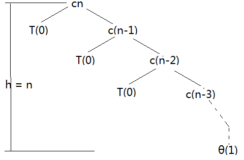
则 cost 为 \(Θ(\sum_{k=1}^nck)=Θ(n^2)\)。
Best-case
情况一:均分数组 \(\frac{n}{2}:\frac{n}{2}\)
此时 \(T(n)=2T(n⁄2)+Θ(n)\),参考主定理,因为 \(f(n)=n=n^{log_2^2}\),属于 case 2,所以 \(T(n)= Θ(nlgn)\)。
情况二:\(\frac{n}{10}:\frac{9n}{10}\)
此时 \(T(n)=T(n/10)+T(9n/10)+θ(n)\)。
递归树分析:
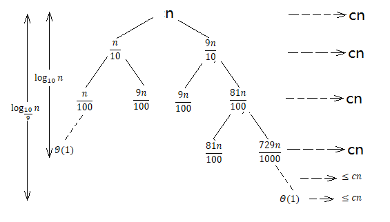 因为下降 step 不同,所以叶节点并不在同一深度。
所以 cost :\(T(n)≤cn⋅log_\frac{10}{9}^n+θ(n)\)。
即 \(T(n)= Ο(nlgn)\)。(a = Ο(b) 类似于 a ≤ b )
事实上,只要划分是常数比例的,算法的运行时间总是 \(T(n)= O(nlgn)\)。
快速排序的 Java 实现
public class QuickSort {

	public static void main(String[] args) {
		int[] arr = {13, 19, 9, 5, 12, 8, 7, 4, 21, 2, 6, 11};
		//quickSort(arr, 0, arr.length - 1);
		quick_Sort(arr, 0, arr.length - 1);
		for (int i = 0; i < arr.length; i++) {
			System.out.print(arr[i] + " ");
		}
	}

	public static void quickSort(int[] arr, int low, int high) {
		if (low < high) {
			int i = low;
			int j = high;
			int x = arr[low];// 选择左边开头的数作为 pivot
			while (i < j) {
				while (i < j && arr[j] >= x)// 从右向左寻找小于主元的数
					j--;
				if (i < j)
					arr[i++] = arr[j];

				while (i < j && arr[i] < x)
					i++;
				if (i < j)
					arr[j--] = arr[i];
			}
			arr[i] = x;
			quickSort(arr, low, i - 1);
			quickSort(arr, i + 1, high);
		}
	}

	public static void quick_Sort(int[] arr, int left, int right) {
		if(left < right){
			int i = partition(arr, left, right);
			quick_Sort(arr, left, i - 1);
			quick_Sort(arr, i + 1, right);
		}
	}

	public static void swap(int[] arr, int i, int k){
		int temp = arr[i];
		arr[i] = arr[k];
		arr[k] = temp;
	}

	/**
	 * partition,左小又大
	 */
	public static int partition(int[] arr, int left, int right){
		int pivot = arr[right];//选择最右边的元素为主元
		int storeIndex = left;
		for (int i = left; i < right; i++) {
			if(arr[i] < pivot){
				swap(arr, i, storeIndex);
				storeIndex ++;
			}
		}
		swap(arr, right, storeIndex);
		return storeIndex;
	}

}
说明: 代码中共有两个快排。
「quickSort(int[] arr, int low, int high)」是常用的快排方法。
「quick_Sort(int[] arr, int left, int right)」主要是用来体现分区的一种写法。
两种写法都可以实现快速排序。
参考
[1] 维基百科 Divide and conquer algorithm.
[2] 麻省理工学院公开课:算法导论.
[3] 维基百科 Master theorem .
[4] 算法导论.第三版第七章:快速排序.
[5] 常见排序算法 - 快速排序 (Quick Sort).
[6] 白话经典算法系列之六 快速排序 快速搞定.
愿你我都是有态度的人,相识于有温度的文字中。
最后,感谢阅读。